I've been playing around for the past few days with other creative ways to utilize the in-cell charting technique I've posted about. Here are two of my current favorites:
1) You can use in-cell charts to create Gantt charts. Let me just say that creating Gantt charts in Excel is hardly breaking any new ground. John Peltier has shown us advanced techniques for doing this using Excel's built in charting feature, and Mr. Excel has shown us how to build Gantt charts using simple conditional formatting. I'm passing this along as just another way to accomplish a similar visual appearance. Below is a small image of what I've done (click on it to open a new window with a larger image):
To create the bars in the chart I use the following formula:

=REPT(" ",D5-G$4)&REPT("█",E5-D5+1)
You can see to accomplish what we need, we first repeat a space (" ") a number of times equal to the start date of the task minus the start of the timeline. Then we repeat ASCII code 219 (hold < ALT > while typing 2 then 1 then 9) a number of times equal to the end date of the task minus the start date of the task + 1. I've also done this one to use conditional formatting to color-code the bars based upon their STATUS. Pretty straightforward, I think.
2) You can use in-cell charting to create graphic displays, such as a graphic equalizer display. Below is a small image of what I've done (click on it to open a new window with a larger image):
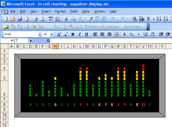
In order to accomplish this look, I have used in-cell charting, only this time I've aligned the "text" (the bar symbols we're using) vertically. Also, since I wanted to have the first 5 bars be green, the next 3 be gold, and the last 2 be red, I've actually split the "bars" into three stacked cells, and adjusted the height of those rows accordingly.
In the lowest segment of each "bar" here's the formula I've used:
=IF(D$8>5,REPT("█",5),REPT("█",D$8))
In the middle segment, here's the formula:
=IF(D$8<6,"",IF(D$8-5>3,REPT("█",3),REPT("█",D$8-5)))
In the topmost segment, here's the formula:
=IF(D$8<9,"",IF(D$8-8>2,REPT("█",2),REPT("█",D$8-8)))
Add to this a little standard formatting with a black background, grey border with diagonal borders drawn on the corners for a 3D effect, and you've got yourself a nice looking graphic equalizer display. The possibilities from here are endless. You could feed this display the bar values dynamically from some other application using VBA, etc.
Additionally, this sort of chart could be used just as well as a regular bar chart in which you want to color-code segments.
I'll be packing up these two sample files and sending them off to my Excel_Geek Insiders subscribers, so you can play around with them and get your own great ideas. Please post a comment on this post if you come up with more cool ideas for in-cell charting.
Later,
Excel_Geek


No comments:
Post a Comment